While Lyapunov fractals have been explored since the early nineties, we now have enough computing power in a desktop PC to start considering them in more than two dimensions. It turns out there’s some weird-looking stuff hanging around in this unexplored parallel world.

This is a piece I wrote back in 2011, and never got around to posting. As I didn’t manage (yet) to bring the work to a conclusion thanks to Real Life™ getting in the way, I didn’t feel it was ready. Please excuse the somewhat fractured tone too; I never really decided what audience I was writing it for. Oh well, screw it.

UPDATE: I’ve released my source code, albeit in a messy barely-working state. Don’t expect much…

(cue wavy flashback effect to 2011 and sepia-toned images)

As I type this, there’s a roaring sound emanating from the hallway. It’s the sound of a bargain basement PC desperately trying to expel hot air quicker than the overburdened graphics card inside can generate. For a while it was under my desk, but my feet got too hot and the sound was unbearable.

Every ten minutes or so, the high-pitched warbling that accompanies the roar drops a little, before cranking back up again. It’s the sound of the fan system taking a quick break while the under-utilised main processor inside the computer wakes up to shift a chunk of freshly-calculated geometric data onto the similarly unburdened hard drive.

By the end of the following day, a couple of gigabytes of this data will have been freshly minted, ready to convert into a hundred-megapixel image with absolutely no practical use whatsoever, other than for me to stare at it, scowl and start staring at the code again, hoping to figure out why it’s either blurry or jagged at a particular point.

Over the past few months, this has been a frequent ritual: stare at a new image, tweak some code for an hour or two, and then start the PC going again on another 100,000-second-long task while I get on with my day job.

Even that’s an improvement, though. Last year, when I started this exercise in distraction and electricity-wastage, a render would take a month to complete, and chances are it’d look terrible in some way after thirty days of anticipation.

The reason I’m doing this is simple: I don’t think anyone else has looked at this particular type of geometry in true 3D before.

It began for me in 1991, when I read an article by A.K. Dewdney in Scientific American. It described a new type of fractal discovered by Dr. Mario Markus of the Max Planck Institute for Molecular Physiology while investigating how enzymes operate in the process of digestion. Like many other mathematical models of real-world processes, it’s chaotic and governed by a simple formula called the Logistic Equation.

This tries to describe the way a simple population of animals grows and shrinks over time. Put simply, the size of next year’s population is a function of the size of this year’s population and a factor denoting the conditions of the environment: how much food is available; how much space is available; how warm it is; and so forth. Typically, winter is a lot harsher than summer, and breeding is affected as a result.

Given poor conditions, a population never thrives and may even die out.

Given good conditions, a population will thrive and will eventually run out of food and space, causing famine. This results in more food and space next year, and the cycle continues: no matter how brutal the famine might be, it can still be stable, oscillating between two wildly different population levels in perpetuity.

If the conditions are just right, the population might settle at a maintainable level without wild swings back and forth.

Regardless, it’s clear that the conditions are critical to the success and failure of the population over the short, medium and long term. The dynamics of the system are fundamentally altered by even the slightest change. In many circumstances, what seems to be a stable population is actually incredibly close to the cliff’s edge.

The exact behaviour can be characterised using the Lyapunov Exponent of the system. This describes how stable or chaotic the system is for a given set of conditions.

The thing is, sometimes the conditions change. The most obvious manifestation of this is the cycle of the seasons: summer and winter are different enough to influence the population of insects and animals significantly. Too many cold winters, and the population dies out. Too many hot summers, and the population goes rampant and ends up dying out too.

So, what’s the ideal combination of winter temperatures and summer temperatures for a given population with a given food supply? Well, there are loads of them, all with their own dynamics.

Back in the eighties, available computing power was just about good enough to start simulating these populations properly, over the digital equivalent of many, many generations. Dr. Markus had the opportunity to visualise these simulations.

The images he created were striking: images of swooping curves and spiky mountain ranges, among a dark sea of noise. The curves signified conditions that would yield a stable situation, while the noise indicated chaotic results where the population would fluctuate so wildly it couldn’t be generalised.

The images were also breathtakingly beautiful — well, for computer graphics in the late eighties, that is. We’d already been wowed by the apple-shaped kaleidoscope of Mandelbrot fractals, but these looked quite different. They looked three-dimensional, even if the mathematics said they were flat as a pancake.

Why were they flat? Well, the algorithm only simulated two variables: A and B. The population oscillated between these two simplified choices. In effect, each image was a chart showing the behaviour of different values of A (up the vertical axis) and B (across the horizontal axis). Each different cyclic pattern of As and Bs gave a different shape to the overall image.

These images evoked a vaguely natural, though not terrestrial feeling. This was more than a simple geometric pattern, and felt a lot more real than the abstract Mandelbrot pattern. It was impossible to look at these new fractals without imagining that they were truly three-dimensional.

When the article in Scientific American came out, I, like many other programmers, had a go creating our own images of this newly-discovered Lyapunov Space. The program was straightforward and included in the article: calculate the Lyapunov Exponent at each point in the image by iterating a simple equation a few thousand times per point. Pick a colour from a simple palette based on the value of the exponent. In many ways, it’s simpler than the Mandelbrot equation, with no imaginary numbers to have to understand. “Simple” doesn’t necessarily mean “easy”, though.

Back then, computing power was still fairly limited for us mere hobbyists. We could get some low-resolution images that looked okay, but it still took hours or days. There was no way we could browse around. If we managed to find a good picture, it was more luck than anything else.

There’s also the fact that two-dimensional Lyapunov space can get pretty boring.

However, there’s an obvious question lurking here: why just two variables? If two variables gives us a two-dimensional image, what does it look like with three variables? Or four?

Fast forward a couple of decades.

We now have far more powerful computers. Heck, even my iPhone could make a fairly good stab at it, considering it’s levels of magnitude faster than the cutting-edge Acorn Archimedes I was using back in 1991.

So, with all this new hardware, what can we see? Two-dimensional Lyapunov fractal code is a standard part of many off-the-shelf fractal packages, and enthusiasts have made some nice art with them. However, it’s still pretty slow: rather than trying it in real-time, we tend to choose to use the extra horsepower to improve quality rather than interactivity.

Looking at the two-dimensional fractal, we can try to imagine it being a thin slice through a three-dimensional fractal instead.

Rather than iterating between A and B, we throw in values for C as well. For any particular slice, C is constant, and we just get a slightly more complex 2D Lyapunov. By changing C for each slice, we can animate smoothly.

No longer is our sweeping curve just a claw-shaped protuberance: it’s now a cross-section through a more complicated shape. Maybe it’s a prismatic shape like the curved aerofoil of a wing, or a bubble, or a landscape, or a cloud. It might still be a claw or sinew, and we just happened to slice that claw down the middle.

Anyway, in lieu of a holographic display, we’ll need a new way to visualise it. I started off by producing a volumetric rendering of the new Lyapunov space.

Volumetric Lyapunov fractals

A standard image — such as a digital photo — is basically a two-dimensional grid of pixels: tiny rectangles of colour. All we need to do is extend this from two to three dimensions. A volumetric image is a three-dimensional grid of voxels: tiny cubes of colour, and as with 2D images, often opacity (or transparency) as well.

The first problem is calculating this data. While the equation’s exactly the same as the old-style 2D images, we now have to calculate a lot more. Let’s say our standard is to render a 1000×1000 or one megapixel image: relatively modest even when compared to the cheap camera that comes with the common mobile phone, let alone the average consumer digital camera. If that takes a few minutes to render, then without optimisation the equivalent 1000×1000×1000 volumetric version is going to take a thousand times longer.

The next problem is how to view the volume once it’s been calculated.

Fortunately, there’s quite a lot of software out there for dealing with volumetric data, mainly because that’s what advanced medical imaging techniques such as CT and MRI scans produce. Unfortunately, the software’s pretty clunky. I’ve watched surgeons battle the user interface while trying to read my CT scans.

Anyway, when you have an MRI scan, the machine virtually slices you up and reconstructs the slices into a 3D chunk of data. To see what’s going on in your body, the diagnostician then needs to take that chunk and delve into the various different densities of skin, muscle, blood, bone and other icky tissue types. While the MRI doesn’t record the colour of the tissue in question as an ideal 3D photograph would, it does record other properties, related to the way the type of tissue reacts to magnetic fields.

As these properties categorise different types of tissue, they can be differentiated in the image: at the most basic, the type of tissue can be denoted by a different colour, just the same way the normal Lyapunov fractal colours chaos and stability with different colours. Even so, when viewed in 3D, the doctor would just see a solid cube of stuff. To be able to look inside, some of the tissue has to be made transparent, leaving just the interesting tissue as opaque.

To view three-dimensional Lyapunov space, we can do the same thing: we arbitrarily say that chaos is transparent, and that we’re interested in the solid surface of stability. We apply a transfer function in the visualisation software. This determines how the range of Lyapunov exponents is rendered: positive exponents are transparent, and negative exponents are solid. We can tweak those values to extract different isosurfaces in the data: effectively isolating different levels of stability and ignoring anything more unstable.

This approach works quite well, but available software is either too domain-specific, or it’s so generalised it’s difficult to control. It’s also relatively slow.

It was good enough, however, to check that this whole endeavour was worth it: the initial volumetric renderings showed a glorious environment… one that deserved investigation.

Point clouds

One thing you tend to realise early on while calculating fractals is that it’s worth storing the intermediate data. You don’t want to throw away a week’s worth of calculation just because it’s a bit dark.

Instead, it’s best to save the raw Lyapunov exponents in a (large!) data file, and subsequently apply a separate process to turn it into a visualisation. The volumetric approach can work with the raw data, applying the transfer function in real-time. Since the data is camera-independent, we can fly around it interactively, move the lights around, and change the opacity of different layers. It does suffer from the fact that even two gigabytes of data — the amount of space to store a low-precision 1000×1000×1000 volume — is going to use up most of the resources of the graphics card and still look pretty chunky. For acceptable quality levels, where the size of the individual voxels is less significant than the size of the pixels on screen, we’d need a cube 4000 units wide: 120 gigabytes of data. Even that wouldn’t allow any appreciable amount of zooming.

Put simply, there’s no way a volumetric approach is going to look good on a present-day desktop computer.

Ray marching

The other alternative is a camera-oriented approach: rather than calculating the fractal data independently of the viewer in an objective manner, we can subjectively calculate only the voxels the viewer can see through their current camera position. We waste no time calculating voxels that are going to be obscured in the final image, and we can use that saving to improve the calculation of the voxels we can see.

In doing so, we sacrifice the ability to freely move around the scene without recalculation, but we’re gambling that we can recalculate quickly enough in real-time.

The most typical method for this kind of approach is that of ray tracing, or more accurately ray marching. This process imagines the viewer to be situated at a single point in space, looking at a virtual rectangle in front of them that represents the image we’re constructing. For every pixel on that image, we fire a beam (or ray) from the viewer’s location through the pixel and continue it on until the ray hits a solid object.

The result is a two-dimensional array of points that represent the surface that the rays hit. At this time we have no idea of the orientation of the surface or the resulting colour: just the “depth” of the surface in relation to the camera. We have no more information than a blind man poking the surface systematically with a very long, thin stick.

Typically in ray tracing, the ray is projected through a simple geometric model of the scene and the exact intersection point of the ray and the object determined by algebraic methods. However, the very nature of a fractal means that an intersection test is usually non-trivial. While a simple pre-calculation of a coarse model might provide a useful approximation, it could easily gloss over a legitimate hit resulting in a grossly simpler model.

Some fractals — such as the Mandelbulb set — can rely on the fact that the fractal surface is connected: there is connectivity between all points of the surface. Unfortunately, Lyapunovs don’t seem to exhibit this property: as slices through a higher-dimensional function, points on the slice do not have to be connected.

This means that there’s no shortcut: we can’t use the result of the trace of a neighbouring pixel to determine an approximation of the current one.

The upshot of this is that to project the ray to the closest opaque intersection, we need to step along the ray in tiny steps and evaluate the fractal function at that point.

In the basic ray marching algorithm, the ray is denoted by this equation:

P(t) = C + t⋅V

where C is the camera position; V is the ray direction vector; and t is the progression variable. At each step of the ray, we increase t by ∂t, and thus advance P along the ray by ∂V.

Typically, we will step the ray tens, hundreds or even thousands of times. The more steps, the less chance of accidentally stepping through a valid but thin membrane, giving rise to a herringbone effect.

Now, at this point I must admit that I am no mathematician. I’m a programmer. I’ve been winging it so far, knowing enough maths to be able to get the code to work, but it’s quite likely I’ve completely fouled up the terminology and explanation.

With that said…

At each point P, we iterate the Lyapunov exponent, l. If the exponent is below (or equal to) the threshold value, we have an intersection. However, in most cases, it will have already punched through the threshold, so we need to reverse and find a better approximation.

To do this, we invert ∂V and scale it down to a smaller step size. We continue until the exponent rises above the threshold, at which point we reverse and scale down again. We keep doing this until the step size is negligibly small: typically about 1/16th of the original step size.

It may also be possible to use the values of P(t-∂t) and P(t) to approximate the intersection point using a simple linear extrapolation. This is risky, as the gradient between the two points may not approximate linearly that well.

Once we’ve got the hit point (or a good enough approximation of it) we need to try to guess a surface normal. It may be possible to differentiate the surface equation for an exact result, but for the time being, it is easy to get a good approximation for finding the gradient surrounding the point as a 3-dimensional vector.

To do this, we find six points surrounding the hit point P on the cardinal directions, infinitesimally spaced around the point: typically about 1% of ∂t around P, and calculate the Lyapunov exponent at those points. At this time in the overall ray function, we’ve already iterated a few thousand times along the ray, so six more calculations will add a negligible load to the processor.

The gradient is calculated by finding the difference between the corresponding cardinal points. So, to find the x-component of the gradient, subtract the Lyapunov exponent of the point to the left of P(t) from the exponent of the point to the right of P(t). Similarly, for the y-component, subtract the exponent of the point below P(t) from the exponent of the point above P(t). For z, subtract in front from behind. The resulting difference vector can be normalised and gives a good surface normal for the intersection point.

This is now enough to complete a rendering of the point: we have the location of the intersection, and the surface normal. We also might have remembered to store something of the transparent points the ray has traversed on the way to the hit point: while the transfer function has determined those points to be transparent as their Lyapunov exponents are above the threshold, we can still accumulate a certain amount of near-threshold exponents and render them as translucent fog.

We can even add a fourth variable, D, varied with time just like we varied C with time in 2D.

So far, these images have been produced as static PNG files, or sequences for combining into videos. It’s a long offline process, and not ideal.

However, with the data being generated on the GPU, we can actually keep it in memory and then render it quickly online.

We can simply pass the intersection point, the surface normal at that point, the camera position and the light position to a shader function such as Blinn-Phong. This will quickly give a semi-realistic lit render of the surface, and we can change the lighting and shading in real-time without recalculating the raw data.

It’s even possible to drive it with a SpaceNavigator 3D Mouse, and fly through the fractal…

As stated before, it’s worth storing the hit data to allow different shader functions to be used.

So…

(cue the return back to 2017, and the reasons why it took me six years to finish this post…)

Where does this leave us?

Well, in 2011, I was managing to get the code to compile to a usable state on Linux and (to a lesser extent) MacOS X. My Mac was never really happy with the GPU running the UI and calculation at the same time, so I would boot it into text-mode Linux; unfortunately, that meant I couldn’t use my main machine for my day job.

The other problem was the division of the code between the user interface using OpenGL, and the calculation engine written with OpenCL. Interoperability between these two remains far harder than it should be. Writing it in GLSL would be an option, but I preferred the idea of separating the practical aspects of displaying pixels from the clean mathematical space, and that division seemed appropriate.

However, there’s the question of whether OpenGL and OpenCL should interoperate directly here. The thing with the ray tracing algorithm used is that it parallelises very well: you could allocate a processing unit for each pixel if you could afford the hardware. Or, use of a distributed computing resource, like Amazon AWS EC2 GPU instances, or even better, a supercomputer. So, locking into direct interoperation between OpenGL and OpenCL via shared texture memory on the same GPU node eliminates the possibility of running it on more than as many GPUs that you can fit in a single PC case.

Instead we’d require a very generic worker package that can be easily compiled and installed on GPU nodes without too many outside requirements; a good front-end client that can consume the data from the allocated calculators; and a scheduler that can manage the producer-consumer relationship.

(In fact, I wrote a proof-of-concept for distributed 2D Lyapunov rendering in 2005, built as screensaver modules for Mac OS X: when active, the screensaver module would call a URL to ask for a parameter block, and would submit the data back. All active screensavers would download and display the shared data as collaborators. It was rudimentary but pretty neat. I got stuck on efficient networking and the limitations of AltiVec on my rather decrepit iBook G4.)

In theory, that’s not actually particularly hard to write. The worker node is straightforward: accept a parameter block from a control node that includes the parameters of the fractal, the camera position and orientation, and the rectangle (and x-y stepping) to calculate. A dumb scheduler could be very simple to write, but it could also be extended to adapt to network conditions, frame rate requirements, worker nodes becoming available or unavailable, and so forth.

And the simple OpenGL client backed with, say, ZeroMQ or nanomsg networking should be fairly easy to write too. It wouldn’t have any concept of Lyapunov fractals, but just a simple camera position and orientation with user controls, and the ability to render pixmap data that comes in from the networking stack.

Unfortunately, this is the part where I fell down, for the simple reason that writing native OpenGL code on macOS nowadays is far harder than it should be for a hobbyist with little spare time. My health (chronic bad back) has steadily declined to the point of needing (more) surgery in early 2017, so spending whatever spare time I do have fighting a neglected and undocumented API doesn’t seem like my idea of fun… if anything, I want to spend the time improving and exploring the algorithm, not the Mac GL driver stack.

Apple’s example code is shockingly weak, and with their own technologies in place — Metal, Swift, and so forth — and their neglect of the desktop platform in favour of mobile, it doesn’t seem to be changing any time soon.

So, to continue I’d expect I’d have to migrate to Linux for maximum interoperability with the prospect of using networked calculation. Or even better, get it working in something like Unity.

What cracks me up is that such a native client and fast network facility for scheduling and rendering arbitrary ray-traced visualisation algorithms sounds like something that’d be really useful. Just slip in a nice, abstract OpenCL program and feed it into whatever borrowed supercomputer nodes you can scavenge, rent or steal, and you can fly through it with the greatest of ease. It’s the kind of project that a student could really pick up and run with.

Anyway, what I have right now is some messy code, and some nice pictures. One day I might find the time to wrangle that code into something more impressive. Fingers crossed…

For more details on the images, check out the contemporaneous Flickr album I built as I was doing the renders.

---

Update, March 2018

I finally bit the bullet and a shiny new Jetson TX2 should be arriving in the next few hours!

However, since ordering it last week I’ve been toying with CUDA on my desktop machine (with a GTX 760 — substantially more powerful than the TX2) and have managed to port the code from OpenCL to CUDA, which should simplify things. It’s not perfect yet, but I am seeing Lyapunovvy results. Although it’ll be slower, it does mean I can dedicate the TX2 to rendering, and explore further. The other benefit of the TX2 is that it’s preinstalled to be an ideal development platform for NVidia, so it should reduce the amount of time wasted doing non-fractal-related debugging.

I’m pushing my changes to the GitHub repo as I’m making them, so I’m hoping I can get it into a fairly cross-platform and easy-to-use form.

Here are a couple of grabs from the CUDA code. As the GPU is also my machine’s UI, it is limited to a short calculation time, so these frames are rendered in less than a second.

I’m intending to write a “snapshot” function to take the current low-res real-time view and file it for high-res high-accuracy (high iteration count) rendering in the background.

---

Update, November 2018

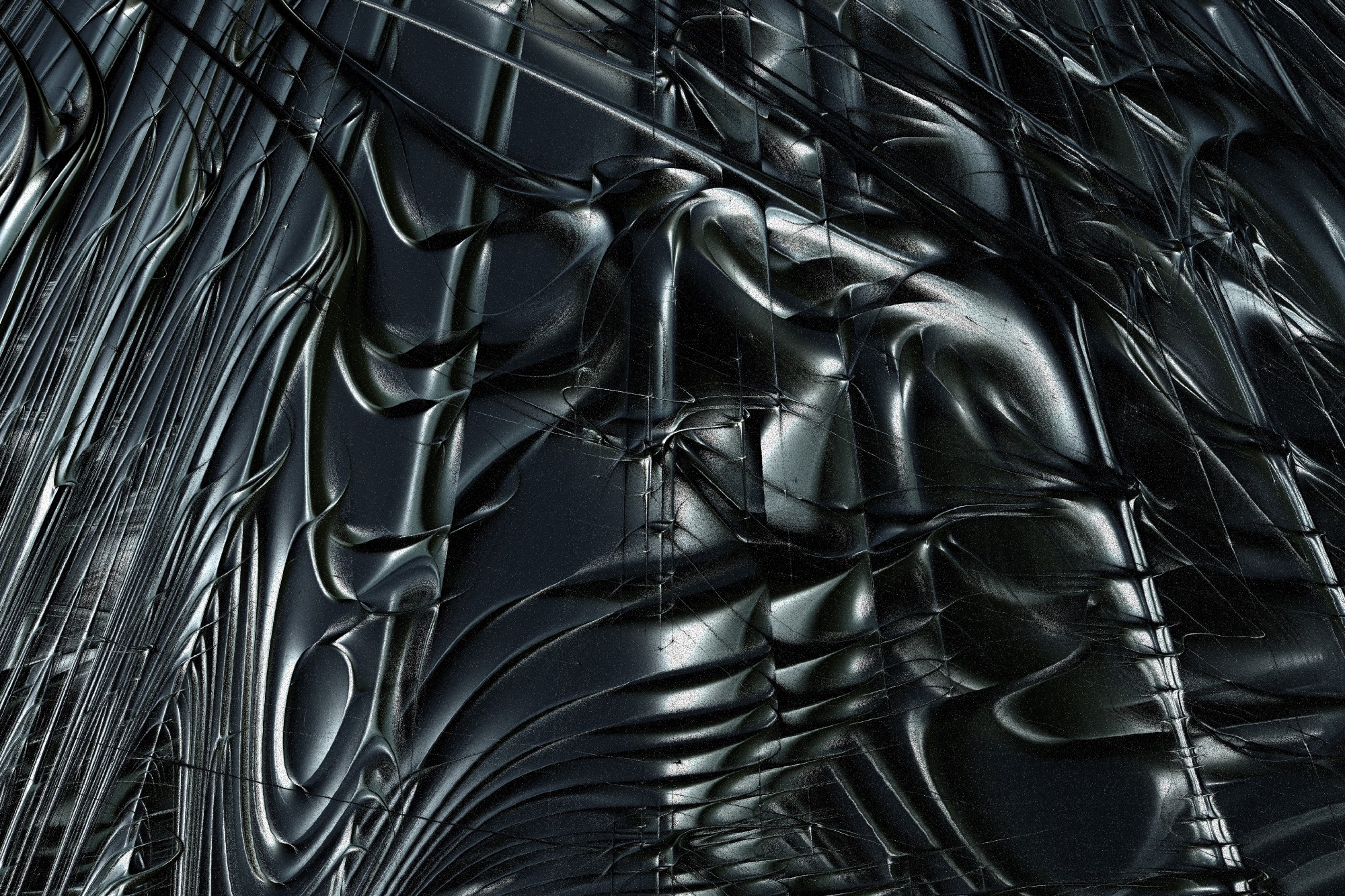
I’ve done another animation render with the new CUDA-based code, rendered at 4K. It’s not perfect, but it’s given me a better idea of how this new code works.

I think for better efficiency I need to learn a lot more about CUDA — in particular to use a producer/consumer model for workers so early terminators are freed up sooner. I’ve also got an idea about how to improve clarity with an accumulative alpha value so membranes (of which I believe there might be infinitely many between any two points!) don’t scruff up the space so much.

The render took about 11 days, about 2–3 hours per frame on a Jetson TX2. As I don’t have an interactive version of this working (at this time) I had to program the quarternion/nlerp-driven camera motion blind, so it’s a little dull.